11 Publishing Analyses to the Web

11.1 Learning Objectives

In this lesson, you will learn:

• How to use git, GitHub (+Pages), and (R)Markdown to publish an analysis to the web

11.2 Introduction

Sharing your work with others in engaging ways is an important part of the scientific process. So far in this course, we’ve introduced a small set of powerful tools for doing open science:

• R and its many packages
• RStudio
• git
• GiHub
• RMarkdown

RMarkdown, in particular, is amazingly powerful for creating scientific reports but, so far, we haven’t tapped its full potential for sharing our work with others.

In this lesson, we’re going to take an existing GitHub repository and turn it into a beautiful and easy to read web page using the tools listed above.

11.3 A Minimal Example

• Create a new repository on GitHub
• Initialize the repository on GitHub without any files in it
• In RStudio,
  • Create a new Project
  • When creating, select the option to create from Version Control -> Git
  • Enter your repository’s clone URL in the Repository URL field and fill in the rest of the details
• Add a new file at the top level called index.Rmd
• Open index.Rmd (if it isn’t already open)

• Press Knit

  Observe the renderd output Notice the new file in the same directory index.html. This is our RMarkdown file rendered as HTML (a web page)
• Commit your changes (to both index.Rmd and index.html)
• Open your web browser to the GitHub.com page for your repository

• Go to Settings > GitHub Pages and turn on GitHub Pages for the master branch

  Now, the rendered website version of your repo will show up at a special URL.

  GitHub Pages follows a convention like this:

  

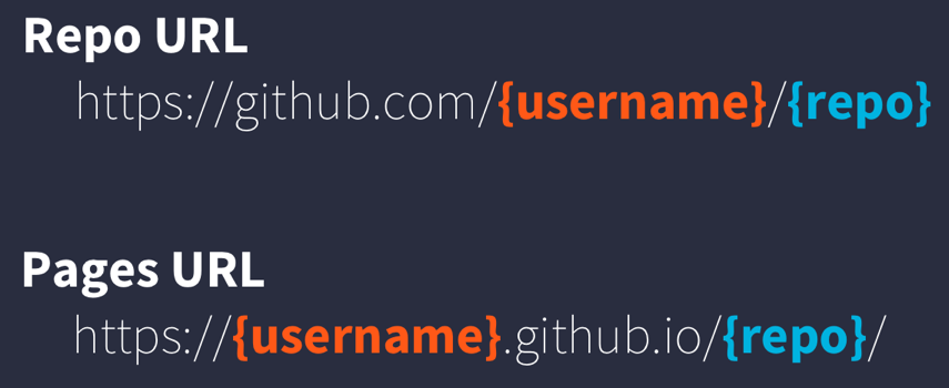
  github pages url pattern

  Note that it will no longer be at github.com but github.io

• Go to https://{username}.github.io/{repo_name}/ (Note the trailing /) Observe the awesome rendered output

Now that we’ve successfully published a web page from an RMarkdown document, let’s make a change to our RMarkdown document and follow the steps to actually publish the change on the web:

• Go back to our index.Rmd
• Delete all the content, except the YAML frontmatter
• Type “Hello world”
• Commit, push
• Go back to https://amoeba.github.io/rmd-test/

11.4 A Less Minimal Example

Now that we’ve seen how to create a web page from RMarkdown, let’s create a website that uses some of the cool functionality available to us. We’ll use the same git repository and RStudio Project as above, but we’ll be adding some files to the repository and modifying index.Rmd.

First, let’s get some data. We’ll re-use the salmon escapement data from the ADF&G OceanAK database we used earlier.

• Navigate to https://knb.ecoinformatics.org/#view/urn:uuid:8809a404-f6e1-46a2-91c8-f094c3814b47 (or visit the KNB and search for ‘oceanak’) and copy the Download URL for the ADFG_firstAttempt_reformatted.csv file
• Make a folder in the top level of your repository to store the file called data

• Download that file into the data folder with the filename escapement_counts.csv

  Note that this is different than how we’ve been downloading data in earlier lessons because we’re actually going to commit the data file into git this time.

• Calculate median annual escapement by species using the dplyr package
• Display it in an interactive table with the datatable function from the DT package

• Make a bar plot of the median annual escapement by species using the ggplot2 package

And lastly, let’s make an interactive, Google Maps-like map of the escapement sampling locations. To do this, we’ll use the leaflet package to create an interactive map with markers for all the sampling locations:

First, let’s load the packages we’ll need:

suppressPackageStartupMessages({
  library(leaflet)
  library(dplyr)
  library(tidyr)
  library(ggplot2)
  library(DT)
})

Then, let’s create the data.frame we’re going to use to plot:

esc <- read.csv(url("https://knb.ecoinformatics.org/knb/d1/mn/v2/object/knb.92020.1", method = "libcurl"), 
                stringsAsFactors = FALSE)

Now that we have the data loaded, let’s calculate median annual escapement by species:

median_esc <- esc %>% 
  separate(sampleDate, c("Year", "Month", "Day"), sep = "-") %>% 
  group_by(Species, Year, Location) %>% 
  summarize(escapement = sum(DailyCount)) %>% 
  group_by(Species) %>% 
  summarize(median_escapement = median(escapement))

ggplot(median_esc, aes(Species, median_escapement)) +
  geom_col() +
  coord_flip()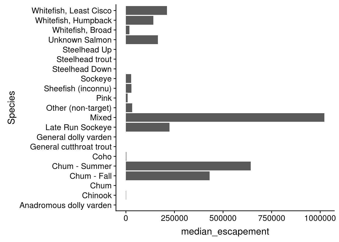

Calculate median annual escapement by species using the dplyr package Let’s convert the escapement data into a table of just the unique locations:

locations <- esc %>% 
  distinct(Location, Latitude, Longitude) %>% 
  drop_na()

And display it as an interactive table:

datatable(locations)

Then making a leaflet map is only a couple of lines of code:

leaflet(locations) %>% 
  addTiles() %>% 
  addMarkers(~ Longitude, ~ Latitude, popup = ~ Location)

The addTiles() function gets a base layer of tiles from OpenStreetMap which is an open alternative to Google Maps. addMarkers use a bit of an odd syntax in that it looks kind of like ggplot2 code but uses ~ before the column names. This is similar to how the lm function (and others) work but you’ll have to make sure you type the ~ for your map to work.

While we can cleary see there are some serious isues with our data (note the points in Russia), this map hopefully gives you an idea of how powerful RMarkdown can be.

Hampton, Stephanie E, Sean Anderson, Sarah C Bagby, Corinna Gries, Xueying Han, Edmund Hart, Matthew B Jones, et al. 2015. “The Tao of Open Science for Ecology.” Ecosphere 6 (July). https://doi.org/http://dx.doi.org/10.1890/ES14-00402.1.

Ioannidis, John P A. 2005. “Why Most Published Research Findings Are False.” PLoS Medicine 2 (8): e124. https://doi.org/10.1371/journal.pmed.0020124.

Ioannidis, John P A, David B Allison, Catherine A Ball, Issa Coulibaly, Xiangqin Cui, Aedín C Culhane, Mario Falchi, et al. 2009. “Repeatability of Published Microarray Gene Expression Analyses.” Nature Genetics 41 (2): 149–55. http://www.ncbi.nlm.nih.gov/pubmed/19174838.

Marwick, Ben. 2017. Rrtools: Creates a Reproducible Research Compendium. https://github.com/benmarwick/rrtools.

Marwick, Ben, Carl Boettiger, and Lincoln Mullen. 2017. “Packaging Data Analytical Work Reproducibly Using R (and Friends).” PeerJ Preprints 5 (August): e3192v1. https://doi.org/10.7287/peerj.preprints.3192v1.

Munafò, Marcus R., Brian A. Nosek, Dorothy V. M. Bishop, Katherine S. Button, Christopher D. Chambers, Nathalie Percie du Sert, Uri Simonsohn, Eric-Jan Wagenmakers, Jennifer J. Ware, and John P. A. Ioannidis. 2017. “A Manifesto for Reproducible Science.” Nature Human Behaviour 1 (1): 0021. https://doi.org/10.1038/s41562-016-0021.

Open Science Collaboration. 2015. “Estimating the Reproducibility of Psychological Science.” Science 349 (6251): aac4716–aac4716. https://doi.org/10.1126/science.aac4716.