Tidy Coral
Julie Lowndes and Jeanette Clark
3/13/2018
Overview
We are going to begin a tidy coral analysis that you will continue on your own. We’ll be using what we learned in the data-science-training but with real coral data from Oahu.
Our plan is to combine benthic observation data with oceanographic buoy data and explore patterns.
We’ll also be using a few new R packages that are super helpful: stringr, janitor, and skimr.
Objectives
- put your data wrangling skills to practice
- read in two real datasets relevant to coral
- join these two datasets together
- learn that this is an iterative process and requires a lot of decisionmaking
Setup
First off, let’s open up a GitHub repo we were working in yesterday, and start a new RMarkdown file. I’ll call mine tidy_coral_analysis.Rmd.
I’ll add a tiny bit of information to get us started, and you can fill in once you know more about what the analysis becomes: “Exploratory analysis to combine benthic observation data with oceanographic buoy data.”
Then we’ll add a setup chunk:
## libraries
library(tidyverse)
library(janitor) # install.packages('janitor')
library(skimr) # install.packages('skimr')
library(stringr) # added when we needed it for benthic data

## data filepaths/urls ----

## benthic data
benthic_url <- 'https://www.nodc.noaa.gov/archive/arc0054/0104255/1.1/data/0-data/cd08/100308OaAla03m.CSV'

## buoy data
buoy_url <- 'http://www.ndbc.noaa.gov/view_text_file.php?filename=mokh1h2010.txt.gz&dir=data/historical/stdmet/'
Benthic data
This is benthic data from a series of CRAMP (Coral Reef Assessment Monitoring Program) data that includes Kaneohe Bay coral survey still images and extracted data (with larger Hawaiian Islands context):
The data we are using resides here.
Import from a URL
Let’s import and have a look with head() and the Environment pane.
benthic_raw <- read_csv(benthic_url)
head(benthic_raw)
There is a lot of columns that are all NA, but let’s not worry about that right now.
Wrangle
Let’s use the janitor package to clean up the column headers. Let’s create a new benthic object with a pipe:
## the `janitor` package's `clean_names` function
benthic <- benthic_raw %>%
  janitor::clean_names()

names(benthic)
## [1] "site_name" "station" "frame_no" "image_date"
## [5] "id_name" "id_code" "point" "x"
## [9] "y" "intensity" "red" "green"
## [13] "blue" "file_name" "total_points" "id_date"
## [17] "site_id" "site_code" "time_code" "institution"
## [21] "user_name" "habitat" "wqs" "length"
## [25] "depth"janitor::clean_names() is such a useful function for taking messy column headers and cleaning them up!
Let’s pull out a few columns that look useful for working with and go from there.
benthic <- benthic %>%
  select(id_name, point, x, y, id_date)

head(benthic)
## # A tibble: 6 x 5
## id_name point x y id_date
## <chr> <int> <int> <int> <chr>
## 1 Pocillopora meandrina 1 1773 1000 #2010-03-12#
## 2 Turf algae 2 2308 194 #2010-03-12#
## 3 Coralline algae 3 1700 1782 #2010-03-12#
## 4 Coralline algae 4 2470 584 #2010-03-12#
## 5 Coralline algae 5 314 1145 #2010-03-12#
## 6 Turf algae 6 198 1660 #2010-03-12#Great. But let’s have another look at those dates. There are some weird #s leading and trailing the dates that will surely cause trouble later, and they don’t look good. So let’s remove them. We can create another column called simply “date”.
Let’s go back up to the setup and add library(stringr) to the setup chunk and run it.
benthic <- benthic %>%
  mutate(date = stringr::str_remove_all(id_date, "#"))
Explore
Now let’s have a quick look at some summary stats:
summary(benthic)skimr::skim(benthic)## Skim summary statistics
## n obs: 4925
## n variables: 6
##
## Variable type: character
## variable missing complete n min max empty n_unique
## date 0 4925 4925 10 10 0 6
## id_date 0 4925 4925 12 12 0 6
## id_name 0 4925 4925 4 21 0 16
##
## Variable type: integer
## variable missing complete n mean sd p0 p25 median p75 p100
## point 0 4925 4925 13 7.21 1 7 13 19 25
## x 0 4925 4925 1271.09 743.82 1 627 1266 1918 2560
## y 0 4925 4925 963.8 546.82 1 489 958 1434 1920
## hist
## ▇▆▆▆▆▆▆▆
## ▇▇▇▇▇▇▇▇
## ▆▇▇▇▇▇▇▇skimr::skim() lets us see quickly that there are 6 unique dates and 16 unique species. It will also make cool histograms of continueous data, although we won’t focus on that at the moment.
Let’s check out which species are represented.
unique(benthic$id_name)## [1] "Pocillopora meandrina" "Turf algae"
## [3] "Coralline algae" "Macroalgae"
## [5] "Montipora capitata" "Montipora patula"
## [7] "Echinometra mathaei" "Porites lobata"
## [9] "Sand" "Substrate"
## [11] "Pavona varians" "Other"
## [13] "Palythoa tuberculosa" "Pavona maldivensis"
## [15] "Pavona duerdeni" "Porites lichen"And to get a sense of our data let’s just have a quick plot of species count by date:
ggplot(benthic, aes(date, fill = id_name)) +
         geom_bar()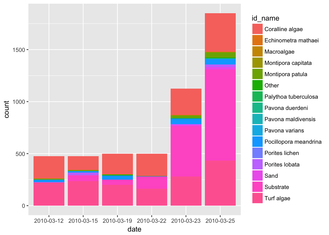
OK so there would be a lot of ways we could improve this plot (starting with color and how it is grouped!). But we just wanted a quick look. And this could help us frame our scientific questions later on. For example:
- why do total counts increase so much through time?
- …
Great! Let’s leave this for a moment and read in the other data.
Buoy data
The buoy data come from the National Buoy Data Center. We are going to use data from the inner Kaneohe Bay buoy (station MOKH1). More details on this station are available here.
Import from a url
Let’s also have a look in the Environment pane as we read in the data.
buoy <- readr::read_csv(buoy_url)
head(buoy) # hmm this doesn't look right! Why not?
Or import a local file!
We could also read this in from a local file if we wanted to. For example:
buoy_raw <- read_csv("data/buoy_local_copy.csv")This imported just as one column. Why didn’t that import properly? Let’s have a look at the URL of the data. Ah right. It’s a .txt, not a .csv.
OK. readr should have a function to read in .txt files. Let’s navigate to the help menu and have a look. In the bottom right RStudio pane, click on “Packages”. Type readr in the search menu, then click on its name. This will let you see all of the functions within the package.
There are a lot of options, but let’s try read_table. It will return a dataframe.
## read_table
buoy_raw <- read_table(buoy_url)
head(buoy) ## still not quite right -- missed some columns.
Why might that be? What is the delimiter for this file? This is when, if I can, I would actually look at the file. I’m going to open the file in a text editor, or even copy-paste a few lines. I use TextWrangler. There, I can “show invisibles” and see what the delimiters are:
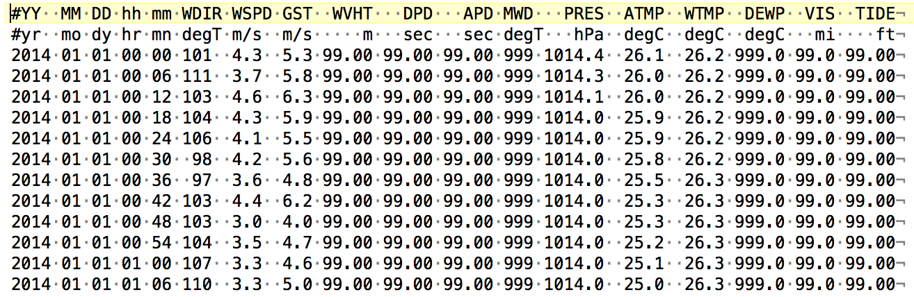
Here the dots show spaces (and a triangle would be a tab, not shown here). So I can see that there is mostly one space separating columns, but there are also up to 5 spaces! This kind of inconsistency can be a problem. This type of file is called a fixed width file.
But…luckily the read_table2() allows for this, because it “allows any number of whitespace characters between columns”. Woop woop!
## read_table2
buoy_raw <- read_table2(buoy_url)
head(buoy_raw) ## this is what we need!
Great, this is what we needed for import!
In creating this tutorial, I actually tried a few other options that didn’t work for various reasons. I spared us from trying this all together (in the interest of time) — but educational to see them and why they didn’t work:
## this just wasn't the right approach
buoy_test <- read_delim(buoy_url, delim = " ", trim_ws = TRUE, skip=1)
This is something I tried to illustrate when you should think to yourself “someone has figured out a better way to do this”. I tried to force it and it involved way too many steps and workarounds, and saving a temporary copy of the data. Boo! This is super unideal. If you find yourself going down a road like this, stop, expect that you’re not the first person to ever access data structured like this, and look for a better way!!!!
buoy_test <- read_lines(buoy_url)
y <- buoy_test %>%
  as_data_frame() %>%
  mutate(value = str_replace_all(value, ' +', ','))
write_delim(y, 'data/buoy_local_copy.csv')

z <- read_csv('data/buoy_local_copy.csv', skip=1)
head(z) ## PRAISE BE
Cool. Nice that read_table2 was designed to get the job done — we just have to expect that it exists and find it.
Wrangle
We’ve got buoy_raw as the raw data we read from online. Let’s create a new variable called buoy that we’ll wrangle instead of that raw data (especially nice if you’ve got poor internet and don’t want to read it in each time!)
buoy <- buoy_rawLet’s look at the column headers.
names(buoy)
head(buoy)
OK. As we know, our data frame needs one column header. But we’ve actually got two rows of information about what the data represent. R thinks that the first row are the column headers, and it considers the second row data. Let’s clean up those names. But we don’t want to lose either of those rows, because they both have important and unique information (measurement and units).
So, let’s see if we can take that the first row of data (the units) and stick it on the with the column names (measurement). Then, we can get rid of that units row.
In the stringr package, there is a way to combine strings using the str_c function.
There’s 3 things we want to do to these column names:
- make the column header a combo of rows 1 and 2
- we want this to look like this:
currentheader_row1. So we want to combine these two rows with a_ - we want to identify row1 by name, not
buoy[1,]because a) it’s cryptic, and b) it will introduce silent problems if you run this code more than once
- we want this to look like this:
- clean up the header; get rid of
#and/ - delete the now-redundant row 1
So let’s start with the first step:
## 1. overwrite column names
names(buoy) <- str_c(names(buoy),                  ## current header
                  buoy %>% filter(`#YY` == "#yr"), ## row1 -- don't say buoy[1,]
                  sep = "_")                       ## separate by `_`

## inspect
names(buoy) ## Looks a lot better
Now the second step:
## 2. clean up a bit more to get rid of the `#`s and the `/`s.
names(buoy) <- str_replace_all(names(buoy), "#", "")  # replace `#` with nothing
names(buoy) <- str_replace_all(names(buoy), "/", "_") # replace `/` with `_`

## inspect to make sure it worked
names(buoy)
Cool, that looks good enough for now!
Final step! Let’s just have a look in the Environment pane to see how many rows there are now (84435 rows, 18 columns)
## 3. remove redundant row with units
buoy <- buoy %>%
  filter(YY_yr != "#yr")
I saw it, did you? In the Environment pane it now says 84434x18. Let’s have another look:
head(buoy)And what would happen if we reran this?
buoy <- buoy %>%
  filter(YY_yr != "#yr")
Nothing, which is great! But if we’d removed buoy[1,], we’d lose a row of data (silently).
Explore
Since we want to analyze these temperatures to the benthic species from above, let’s get a visual of what the temperature data looks like, and then we’ll think about how this relates with the benthic species.
Temperature
ggplot(buoy, aes(WTMP_degC)) +
  geom_bar()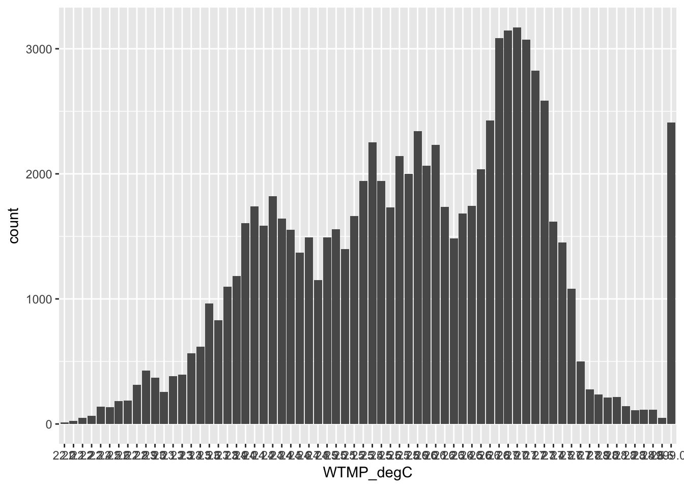
## I googled how to rotate the tick label axis so that we can read the labels:
ggplot(buoy, aes(WTMP_degC)) +
  geom_bar() +
  theme(axis.text.x = element_text(angle = 90))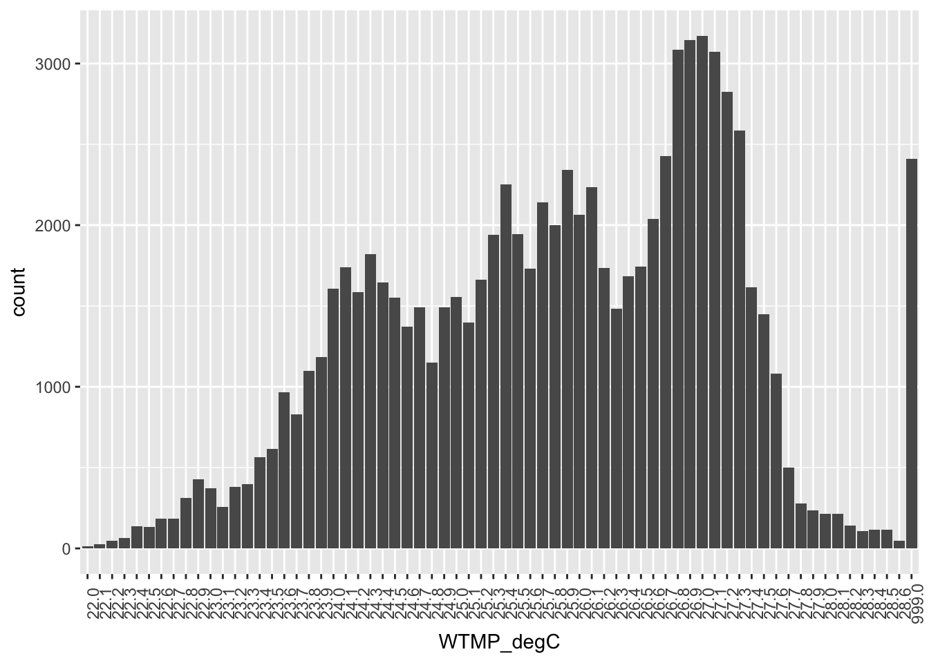
OK. So there is a lot to take in here.
Consider this a to do list when you start working on your own.
- Seems like 999.0 is not really a measured °Celsius
- After confirming with the metadata, we should replace it with NA
stringr::str_replace_all()
WTMP_degCdoes not seem to be numeric (since 999.0 is right there next to 28.6).
- We could confirm this with
str(buoy), then convert to numeric withbuoy <- buoy %>% mutate(WTMP_degC = as.numeric(WTMP_degC)) - Why is this a string? So actually all variables in
buoyare character instead of numeric, and it’s because when we originally read in the file the first row was measurement units, which was a character string. So any of these that we want to treat of numbers we are going to have to explicitly change to numeric.
Dates
Let’s have another look at the dates in buoy, because this is probably how we’re going to join to the benthic data. As a reminder:
head(benthic)
head(buoy)
So the date formats are different between these two datasets, and so we can’t join them as-is. Benthic’s date format is 2010-03-12 and in the buoy dataset it is spread across 3 columns (and also has hours and minutes).
So before we can join we need to wrangle those buoy dates. We know the format we want them to look like, so we can combine them into a new column named date using tidyr::unite(). When we unite these columns it will actually replace the original columns with out new column:
buoy <- buoy %>%
  unite(date, c(YY_yr, MM_mo, DD_dy), sep = "-")

head(buoy)
## # A tibble: 6 x 16
## date hh_hr mm_mn WDIR_degT WSPD_m_s GST_m_s WVHT_m DPD_sec APD_sec
## <chr> <chr> <chr> <chr> <chr> <chr> <chr> <chr> <chr>
## 1 2010-01-01 00 00 999 99.0 99.0 99.00 99.00 99.00
## 2 2010-01-01 00 06 999 99.0 99.0 99.00 99.00 99.00
## 3 2010-01-01 00 12 999 99.0 99.0 99.00 99.00 99.00
## 4 2010-01-01 00 18 999 99.0 99.0 99.00 99.00 99.00
## 5 2010-01-01 00 24 999 99.0 99.0 99.00 99.00 99.00
## 6 2010-01-01 00 30 203 2.1 3.9 99.00 99.00 99.00
## # ... with 7 more variables: MWD_deg <chr>, PRES_hPa <chr>,
## # ATMP_degC <chr>, WTMP_degC <chr>, DEWP_degC <chr>, VIS_nmi <chr>,
## # TIDE_ft <chr>Join datasets
Great, let’s join these datasets!
We can use RStudio’s data wrangling cheatsheet as a reminder:
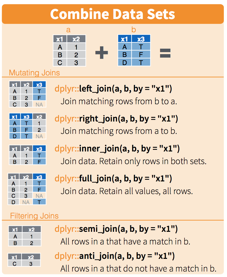
Let’s go with left join by date:
bb_join <- benthic %>%
  left_join(buoy, by = "date")
Woah, just from the Environment pane we can see there are A LOT of observations based on this join. What happened? Let’s have a look:
head(bb_join) # kind of hard to see what's going on.## let's select a few columns and inspect:
bb_join %>%
select(id_name, x, y, date, hh_hr, mm_mn, WTMP_degC) %>%
head()## # A tibble: 6 x 7
## id_name x y date hh_hr mm_mn WTMP_degC
## <chr> <int> <int> <chr> <chr> <chr> <chr>
## 1 Pocillopora meandrina 1773 1000 2010-03-12 00 00 23.2
## 2 Pocillopora meandrina 1773 1000 2010-03-12 00 06 23.2
## 3 Pocillopora meandrina 1773 1000 2010-03-12 00 12 23.2
## 4 Pocillopora meandrina 1773 1000 2010-03-12 00 18 23.2
## 5 Pocillopora meandrina 1773 1000 2010-03-12 00 24 23.2
## 6 Pocillopora meandrina 1773 1000 2010-03-12 00 30 23.2OK, so because the buoy data has sampling every 6 minutes, there is a lot of repeated data as a result of the join. Is that what we want? If not, what should we do?
We could summarize the buoy data by hour or day, or filter the hours that the benthic survey took place. What we do will depend on the science questions you are asking!
Your turn
Save, commit, and sync your work. Then, continue the analysis based on what you’re interested in. Here are some ideas:
Explore benthic data
- what other ways could you visualize the data? What questions does bring up?
Explore buoy data
What are some other things we could do to this data?
- Seems like 999.0 is not really a measured °Celsius
- After confirming with the metadata, we should replace it with NA
stringr::str_replace_all()
- After confirming with the metadata, we should replace it with NA
WTMP_degCdoes not seem to be numeric (since 999.0 is right there next to 28.6).- We could confirm this with
str(buoy), then convert to numeric withbuoy <- buoy %>% mutate(WTMP_degC = as.numeric(WTMP_degC)) - Why is this a string? So actually all variables in
buoyare character instead of numeric, and it’s because when we originally read in the file the first row was measurement units, which was a character string. So any of these that we want to treat of numbers we are going to have to explicitly change to numeric.
- We could confirm this with
- How would you plot a timeseries of temperature change?
Explore joined data
- what variables should you compare? Temperature?
- should you summarize species counts first?
Explore beyond
- Compare a different buoy and benthic pair?
Troubleshooting
tidyverse stringi bug with R version 3.4.3
Our fix for now: uninstall tidyverse, and individually install readr, dplyr, tidyr, and then not stringr; instead, use base-R. So, use the following commands:
To install and load packages:
## uninstall packages
remove.packages('tidyverse')
remove.packages('stringi')
remove.packages('stringr')

## install individual packages
install.packages('readr')
install.packages('dplyr')
install.packages('tidyr')

## load individual packages
library(readr)
library(dplyr)
library(tidyr)
Here is gsub not stringr:
## not str_remove_all...
benthic <- benthic %>%
  mutate(date = stringr::str_remove_all(id_date, "#"))

## ...use gsub instead
benthic <- benthic %>%
  mutate(date = gsub("#","", id_date))

## not str_replace_all...
names(buoy) <- str_replace_all(names(buoy), "#", "")

## ...use gsub instead
names(buoy) <- gsub("#", "",names(buoy)) # replace `#` with nothing